Chapter 50 — Economic Development
Cambridge International AS & A Level Economics (9708) · Unit 11.3 · 4th edition coursebook
Learning objectives
- Describe how economies are classified in terms of their level of development and level of national income.
- Evaluate indicators of living standards and economic development including real per capita national income statistics, purchasing power parity, non-monetary indicators and composite indicators.
- Explain the Kuznets curve.
- Compare economic growth rates and living standards over time and between countries.
Key terms
- poverty cycle
- The links between, for example, low income, low savings, low investment and low productivity.
- development traps
- Restrictions on the growth of developing economies that arise from low levels of savings and investment.
- purchasing power parity (PPP)
- A way of comparing international living standards by using an exchange rate based on the amount of each currency needed to purchase the same basket of goods and services.
- Human Development Index (HDI)
- A composite measure of living standards that includes GNI per head, education and life expectancy.
- Measurable Economic Welfare (MEW)
- A composite measure of living standards that adjusts GDP for factors that reduce living standards and factors that improve living standards.
- Multidimensional Poverty Index (MPI)
- A composite measure of deprivation in terms of the proportion of households that lack the requirements for a reasonable standard of living.
- Kuznets curve
- A curve that shows the relationship between economic growth and income inequality.
- shadow economy
- The output of goods and services hidden from the authorities.
50.1How economies are classified in terms of development and national income
Economies can be grouped according to how developed they are. Highly developed economies typically have high incomes, mature markets, high standards of living and high productivity.
Developed and developing economies
One traditional division is between developed economies — usually with high income per head, well-established economic institutions, advanced technological infrastructure and a strong tertiary sector — and developing economies, typically with lower income per head, reliance on fewer products, a larger primary sector and lower productivity. Some institutions, including the World Bank, and some economists no longer use these labels, because in a sense every economy is developing or trying to develop. Instead they classify economies by the level of development reached (for example by HDI, covered in Section 50.2) or by income per head.
Classification according to income
The most common income-based classification compares GDP per capita, GNI per capita or NNI per capita. The World Bank uses GNI per capita to place each country into one of four bands: low-income, lower middle-income, upper middle-income and high-income. Countries can move between bands as their economies grow or contract. The thresholds between bands are updated each year to keep them constant in real terms.
Income-based classification is straightforward and helps identify countries that need aid. It is also used by the World Bank to set the interest rate it charges on loans — a higher rate for countries that have been classified as high-income for two consecutive years. However, the classifications can mislead, because economies grow and contract over time, and income per head does not capture every influence on development.
Poverty cycles and development traps
Some low-income economies suffer from poverty cycles (see Figure 50.4) that produce development traps. One common cycle runs: low incomes → low savings → low investment → low productivity → low incomes again. A second cycle runs through human capital: low incomes → low levels of education and healthcare → low levels of human capital → low economic growth → low incomes. These self-reinforcing loops mean that growth and development can stall unless the cycle is broken — for example by an inflow of investment, foreign aid, education spending or improvements in healthcare.
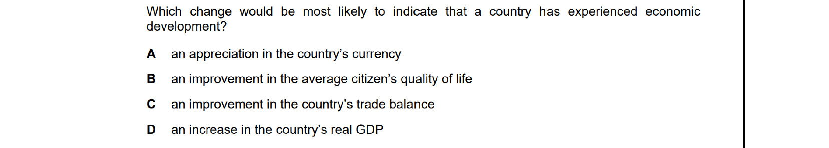
Real GDP, currency appreciation and a better trade balance describe growth or external balance — none guarantees that ordinary people are better off. Economic development is about widening citizens' choices: longer, healthier, better-educated lives. So a clear improvement in the average citizen's quality of life is the surest indicator that development — not just growth — has taken place.
50.2Other indicators of living standards and economic development
To assess living standards and economic development, economists draw on a wide range of indicators. Some are monetary indicators (GDP, GNI, NNI and purchasing power parity comparisons covered in Section 50.3). Others are non-monetary indicators, including infant mortality rates, the number of doctors per 1000 people, literacy rates, and access to clean water. A third group of measures are composite indicators that combine several indicators of living standards and development with weightings to produce a single, combined figure.
Monetary measures alone are limited. They average across the whole population and do not show how income is distributed, they ignore non-marketed activity, and they say nothing about education, health or environmental quality. Composite measures attempt to remedy these weaknesses by drawing in information on outcomes that matter for welfare.
Human Development Index
The best-known composite measure is the United Nations' Human Development Index (HDI). It combines three components:
- GNI per head (as a measure of command over goods and services);
- Education, measured by two figures combined: expected years of schooling for a child of school entrance age, and mean years of schooling for adults aged 25 and above;
- Health, measured by life expectancy at birth.
The reasoning is that welfare depends not only on the goods and services available to people but also on their ability to lead a long, healthy life and to acquire knowledge. The HDI is expressed as a value between 0 and 1, with 1 the maximum possible. The value can be read as the distance a country still has to cover to reach that maximum. Countries are then grouped into four bands: very high, high, medium and low human development.
A country's HDI ranking does not always match its GNI per head ranking. Some countries do markedly better on HDI than on income, because they have invested heavily in education and health relative to their income level. Others do worse on HDI than on income, because high incomes have not translated into the same gains in life expectancy and schooling. Remember when answering questions on the HDI that life expectancy is influenced by healthcare, but what is actually measured is life expectancy itself, not the quality or quantity of healthcare.
Measurable Economic Welfare
Measurable Economic Welfare (MEW) was developed by economists to try to give a fuller picture of living standards by adjusting GDP for items GDP misses. Factors that improve living standards - for example, increased leisure time - are added to the GDP figure. Factors that reduce living standards - for example, environmental damage - are deducted. In practice, valuing non-marketed goods and bads is difficult and expensive, which limits how widely MEW can be applied.
Multidimensional Poverty Index
The Multidimensional Poverty Index (MPI) was developed by international development bodies to measure poverty across multiple dimensions. It measures ten indicators across three dimensions:
- Living standards (six indicators): cooking fuel, sanitation, drinking water, electricity, housing and assets;
- Education (two indicators): years of schooling and school attendance;
- Health (two indicators): child mortality and nourishment.
The three dimensions each carry a weighting of one-third. Within each dimension, the indicators share the weight equally. A household is judged to be multidimensionally poor if it is deprived in at least one-third of the weighted indicators - for example, a family that has lost a child and has another child who is not attending school.
The aim of the MPI is to help countries understand why people are poor and why some stay poor even when incomes rise. By drilling beneath an average income figure, the MPI helps governments and international organisations target the poorest groups, assess progress, and co-ordinate national development plans.
The Kuznets curve
The Kuznets curve (see Figure 50.6) suggests an inverted-U relationship between income per head and income inequality. As an economy starts to develop from a low base, income becomes more unevenly distributed. After a certain income level is reached, income then becomes more evenly distributed again. Plotted with GDP per head on the horizontal axis and income inequality (for example the Gini coefficient) on the vertical axis, the curve rises first and then falls.
The proposed reason for the initial rise in inequality is structural. As an economy develops, labour gradually moves from low-paid, low-skilled agricultural jobs into higher-paid, more skilled manufacturing jobs. Workers who move first capture the higher wages, while those still in low-paid sectors do not; the gap between the two groups widens. Eventually, as more workers move into the higher-paid sectors and as education, taxation and welfare systems spread the gains more widely, inequality begins to fall.
The pattern is not seen everywhere. Some developing economies have experienced rising inequality without the predicted later fall, and the curve does not explain the rise in income inequality observed in some high-income economies. The Kuznets curve is therefore a useful stylised description rather than a reliable forecasting tool.
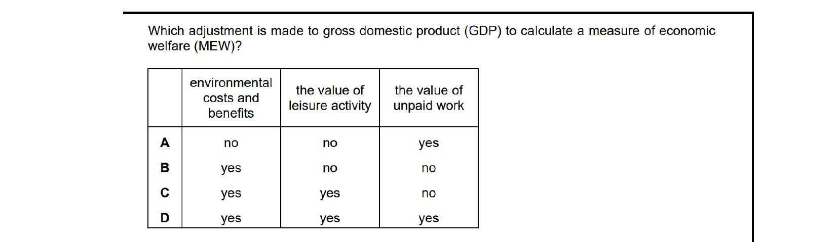
The Measure of Economic Welfare adjusts GDP for items it ignores. It subtracts environmental costs (and adds environmental benefits), adds the value of leisure activity, and adds the value of unpaid work (e.g., household production). All three adjustments are made, so option D correctly says yes to environmental costs/benefits, leisure and unpaid work.
50.3Comparison of economic growth rates and living standards
Economic growth rates are calculated from changes in real GDP, GNI or NNI between two periods. International league tables routinely report these figures side by side. Comparing growth rates over time and between countries is, however, more difficult than it sounds, and the difficulties multiply when growth rates are translated into claims about living standards.
The shadow economy
One difficulty is the shadow economy - undeclared economic activity, also known as the hidden or underground economy. People hide income for two main reasons. The first is to evade tax: a tradesperson, for example, may take cash for spare-time work and not declare it. The services produced are real, but the income, and therefore the output, never enters the official statistics. The second is that the activity is itself illegal, such as smuggling.
One way to estimate the size of the shadow economy is to compare GDP measured by the expenditure method with GDP measured by the income method, because people will still spend income they have not declared - the gap between the two measures hints at the size of the hidden activity.
If the shadow economy is roughly constant in size, the official growth rate can still be reasonably accurate, because the same proportion is missing in both periods. But the size of the shadow economy varies between countries, depending on marginal rates of taxation, the penalties imposed for evasion and illegal activity, the risk of being caught, and social attitudes to particular activities. This variation makes international comparisons of growth rates much harder.
Other measurement problems
Official figures may also fail to capture output and changes in output accurately for other reasons:
- Low levels of literacy: some people cannot complete tax forms, and others complete them inaccurately, so the authorities must estimate some output.
- Non-marketed goods and services: GDP includes only items that are bought and sold and so have a price attached. Goods and services produced and either not traded or exchanged without money changing hands - domestic services within the home, painting and repairs by home-owners, voluntary work - go unrecorded. The amount of self-production and voluntary work varies over time and between countries.
- Government spending: it is difficult to measure the value of services provided by the public sector, since they are often supplied free or at a price that does not reflect their value.
The nature of growth
When comparing growth rates it is also important to consider the nature of growth. A very high growth rate may initially look impressive, but it may not be sustainable if it depletes non-renewable resources or generates pollution that lowers the fertility of the land and the health of the labour force. A slower growth rate based on renewable resources, cleaner production and rising productivity may deliver more welfare in the long run than a higher rate built on resource depletion.
Comparison of living standards over time
Real GDP per head has traditionally been one of the main indicators of living standards. If a country's real GDP per head is higher this year than last, it is generally expected that average living standards are rising. This is often true, but not always.
Real GDP per head is calculated by dividing total real GDP by the population. As an average, it does not capture how output is distributed. If the gains from growth accrue mainly to a small group, the average can rise while many people see their incomes stagnate or fall. Changes in the shadow economy over time also distort the link between measured GDP and what households actually consume.
To assess changes in living standards, the composition of output also has to be considered. During a war, output rises because more weapons are produced, but few would say that living standards have improved. Recruiting more police to deal with rising crime increases real GDP but does not make the population feel better off. By contrast, more consumer goods and services - housing, food, clothing, transport - do raise living standards directly.
A shift of resources from consumer goods to capital goods is a special case (see Figure 50.8). In the short run, if the economy is operating on its production possibility frontier, fewer consumer products will be enjoyed today. In the long run, the higher capital stock raises productive capacity, so more consumer products can be produced and enjoyed later.
Even when people enjoy more consumer goods and services, it does not necessarily mean they will be happier. As access to more and higher-quality products rises, the desire for still more and better products may rise even faster, so subjective well-being need not improve.
Real GDP measures the quantity of output, not its quality. If quality falls, living standards fall even though GDP does not. In practice, the quality of output tends to rise over time, which means living standards can rise even when real GDP per head is roughly constant. Working conditions also tend to improve over time and working hours tend to fall: if real GDP per head stays the same but workers enjoy shorter hours and safer conditions, living standards have improved.
Environmental degradation lowers living standards but may not lower real GDP. Pollution, deforestation and the loss of natural capital harm welfare directly, and if more resources have to be devoted to cleaning up the environment, GDP rises while living standards decline.
Comparison of GDP per head and living standards between countries
The citizens of a country with a higher GDP per head are likely to enjoy higher living standards than those in a country with a lower GDP per head - but this is not guaranteed.
To compare living standards between countries, real GDP per capita has to be converted into a common currency. To avoid the comparison being distorted by exchange rate movements, economists usually adjust exchange rates using purchasing power parity (PPP). PPP uses an exchange rate based on the amount of each currency needed to buy the same basket of goods and services, rather than the market exchange rate.
A numerical illustration. Suppose the market exchange rate is 6 units of country B's currency to $1, country A has a real GDP per head of $50000, and country B has a real GDP per head of 12000 units of its currency. Converted at the market rate, country B's output looks like just $2000 per head - so country A appears 25 times better off. But suppose a basket of goods costing $200 in country A costs only 2400 units of B's currency in country B. The PPP exchange rate is then 12 units per $1 (2400/200), not 6. Using the PPP rate to convert country B's output makes country A appear 50 times better off than country B in terms of actual purchasing power. Where the market rate diverges from the PPP rate, raw GDP comparisons will overstate or understate one country's real output relative to the other.
A widely cited simplified version is the Big Mac index published by The Economist. It compares the price of a Big Mac across countries to back out an implied purchasing-power exchange rate, and then compares this to the market exchange rate. If, for example, a Big Mac costs $4 in one country and the equivalent of £3 in another, the implied PPP rate is £1 = $1.33. If the actual market rate is £1 = $1.50, the pound looks overvalued and may fall in future. The Big Mac index trades accuracy for clarity, but it makes the basic logic of PPP easy to communicate.
Even after adjusting for PPP, a higher real GDP per head does not guarantee higher living standards. Where income is very unevenly distributed, only a small share of households may benefit from a high average. Other factors not captured in GDP - working hours, working conditions, fear of crime, freedom of thought, environmental quality - matter just as much when comparing between countries as when comparing over time.
It is useful to include a numerical example in any answer that explains purchasing power parity.
Key concept link - Progress and development
Economies make progress if their residents can enjoy a higher quality of life.
Key concept link - Efficiency and inefficiency
A good standard of living can promote efficiency as it is likely to make workers more productive.
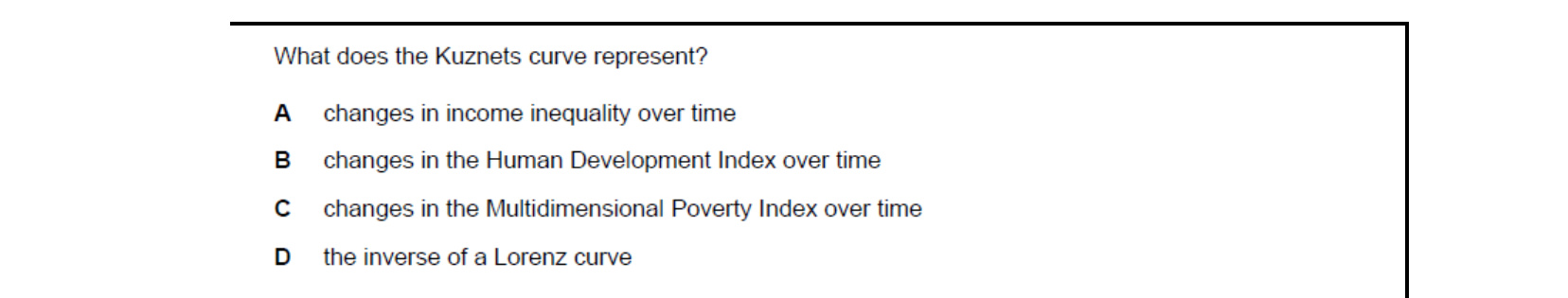
The Kuznets curve is an inverted-U showing how income inequality first rises as a country industrialises and then falls as development matures. It plots changes in income inequality over time, not HDI, MPI or the Lorenz curve — so option A captures what the curve represents.
End-of-chapter practice
Past-paper questions from CIE 9708. Pick A, B, C or D. Answers are saved on this device — press Download report (PDF) at the top to save them.
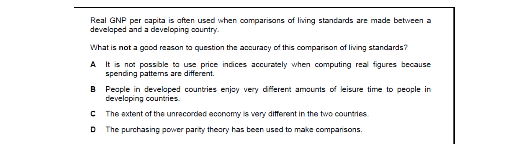
Real GNP per capita has well-known weaknesses for cross-country comparisons: different consumption patterns make price indices imperfect (A); leisure time differs (B); and the size of the informal/unrecorded economy varies (C) — all good reasons to doubt the comparison. Using purchasing power parity, however, is meant to improve comparability. So D is NOT a good reason to question accuracy.

The Kuznets curve plots income inequality against the level of income per head as a country develops: inequality rises in the early stages of industrialisation, then falls once incomes are high enough for redistribution and broader participation. It is not about devaluation, growth rates or tax revenue. So C — the rise then fall in inequality as income per head rises — is correct.
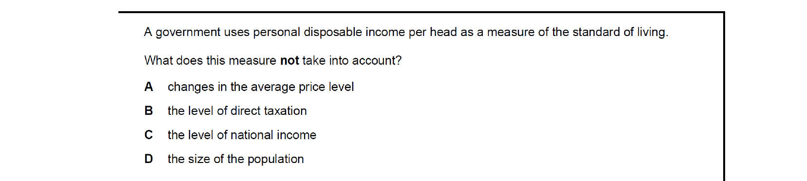
Personal disposable income per head already nets off direct tax (B), accounts for total national income relative to the number of people (C and D). What it does not do is adjust for changes in the price level — nominal disposable income can rise even though real purchasing power falls if inflation outpaces it. So changes in the average price level are missed.
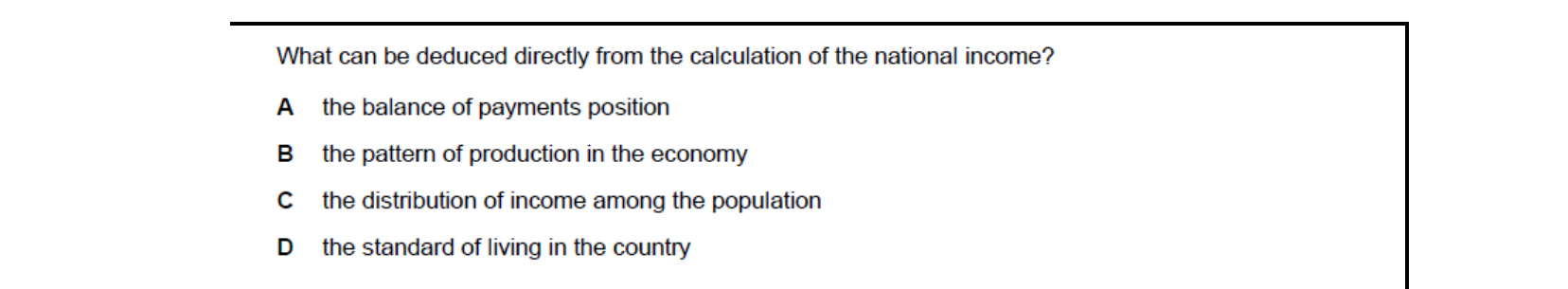
National income statistics record output by sector — agriculture, industry and services — and so reveal the pattern of production in the economy. They do not directly show the balance of payments, the distribution of income across households, or the standard of living (which depends on prices, leisure, public services etc.). The direct deduction is the structure of production.
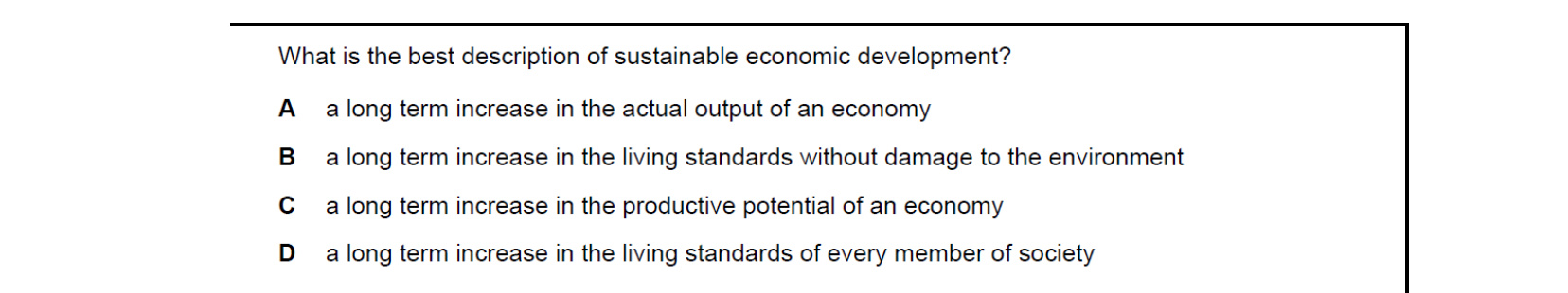
Sustainable development means improvements in living standards today that do not compromise the ability of future generations to enjoy similar improvements — typically by avoiding environmental damage. A long-term rise in actual output, productive potential, or every individual's living standards does not capture the environmental condition. Only B explicitly couples rising living standards with no environmental damage.
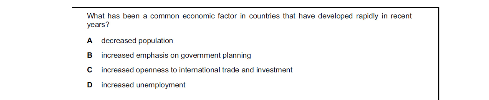
The countries that have grown fastest in recent decades — China, Vietnam, Singapore, the East Asian tigers — opened up to trade and FDI rather than retreating from world markets. Greater openness widens markets, brings in capital, technology and know-how, and disciplines firms via competition. Falling populations, more state planning and higher unemployment are not associated with rapid catch-up.
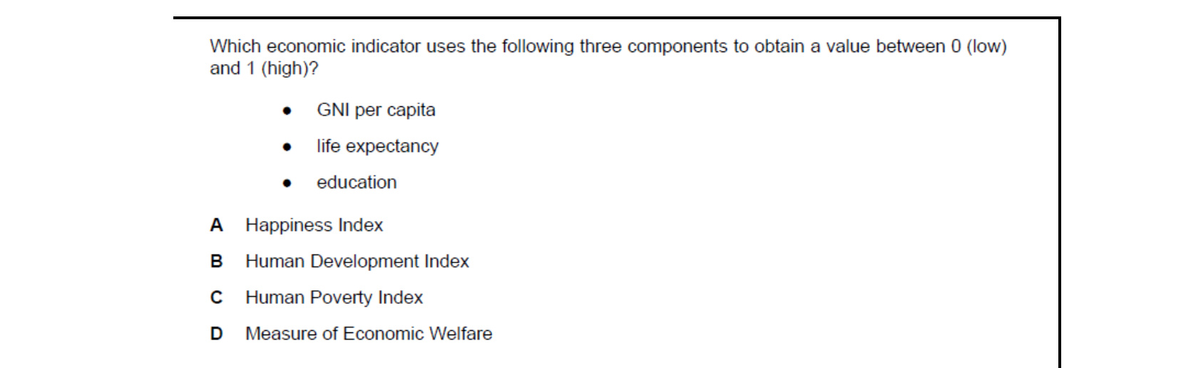
The Human Development Index combines exactly the three indicators listed: GNI per capita (income), life expectancy (a long, healthy life) and education (years of schooling). It is scaled between 0 and 1. The Happiness Index and Measure of Economic Welfare use different components, and the Human Poverty Index focuses on deprivation rather than scoring achievement.
Attempt the practice questions above to build your score.
Self-evaluation checklist
After studying this chapter, you should be able to:
- Describe how economies are classified in terms of their level of development and level of national income.
- Evaluate indicators of living standards and economic development using monetary terms (GDP, GNI, NNI, purchasing power parity), non-monetary terms (such as infant mortality rates) and composite indicators (HDI, MEW, MPI).
- Explain that the Kuznets curve (U-shaped) suggests that as an economy develops, income becomes more unevenly distributed and then after a certain income level is reached, income becomes more evenly distributed.
- Compare economic growth rates over time and between countries using real GDP, GNI and NNI.
- Compare living standards over time and between countries using real GDP.
Want more practice? Drill this chapter's past-paper MCQs (103 questions) →