Chapter 34 — Types of Cost, Revenue and Profit, Short-Run and Long-Run Production
Cambridge International AS & A Level Economics (9708) · Unit 7.5 · 4th edition coursebook
Learning objectives
- Explain the short-run production function, including: fixed and variable factors of production; total product, average product and marginal product; the law of diminishing returns (law of variable proportions).
- Calculate total product, average product and marginal product.
- Explain the short-run cost function, including: fixed costs (FC) and variable costs (VC); total, average and marginal costs (TC, AC, MC); the shape of short-run average cost and marginal cost curves.
- Calculate fixed costs and variable costs, and total, average and marginal costs.
- Explain the long-run production function, including no fixed factors of production and returns to scale.
- Explain the long-run cost function, including the shape of the long-run average cost curve and the minimum efficient scale.
- Analyse the relationship between economies of scale and decreasing average costs.
- Explain internal economies of scale and external economies of scale.
- Explain internal diseconomies of scale and external diseconomies of scale.
- Define the meaning of total, average and marginal revenue.
- Calculate total, average and marginal revenue.
- Define the meaning of normal, subnormal and supernormal profit.
- Calculate supernormal and subnormal profit.
Key terms
- economies of scale
- The benefits gained from falling long-run average costs as the scale of output increases.
- isoquant
- A curve showing combinations of labour and capital to produce a given level of output.
- total product
- The same as total output.
- production function
- The maximum possible output from a given set of factor inputs.
- marginal product
- The change in output arising from the use of one more unit of a factor of production.
- law of diminishing returns
- Where the output from an additional unit of input leads to a fall in the marginal product; also known as the law of variable proportions.
- average product
- Total product divided by the number of workers employed; a simple measure of productivity.
- profit maximisation
- The assumed objective of a firm; the difference between total revenue and total cost is at a maximum.
- fixed costs (FC)
- Costs that are independent of output in the short run.
- variable costs (VC)
- Costs that vary directly with output in the short run.
- increasing returns to scale
- Where output increases at a proportionately faster rate than the increase in factor inputs.
- decreasing returns to scale
- Where factor inputs increase at a proportionately faster rate than the increase in output.
- isocosts
- Lines of constant relative costs for factors of production.
- minimum efficient scale
- Lowest level of output at which costs are minimised.
- diseconomies of scale
- Where long-run average costs increase as the scale of output increases.
- external economies of scale
- Cost savings accruing to all firms as the scale of the industry increases.
- total revenue (TR)
- A firm's total sales or earnings over a given period of time.
- average revenue (AR)
- Revenue per unit of output.
- marginal revenue (MR)
- The additional or extra revenue gained from the sale of one more unit of output.
- price taker
- A firm that is not able to influence market price.
- price maker
- A firm that can choose what price to sell its goods in the market.
- profit
- The difference between total revenue and total costs.
- normal profit
- A cost of production that is just sufficient for a firm to keep operating in a particular industry.
- supernormal profit
- That which is earned above normal profit.
- subnormal profit
- That which is earned below normal profit.
34.1Introduction to production
The demand for the four factors of production — land, labour, capital and enterprise — is a derived demand. Firms want factors not for their own sake but in order to produce goods and services for sale. The most important decision a firm makes is the relative mixture of labour and capital it will use, because in most production processes labour and capital are in direct competition with each other. Where labour is relatively cheap, production tends to be labour-intensive; where labour is relatively expensive, firms substitute towards more capital-intensive methods. Clothing is a familiar illustration: the same output can be produced using many workers and little capital in a low-cost economy, or with high-tech machines and few workers in a high-income economy (see Figure 34.3).
Different combinations of labour and capital can produce the same level of output. A diagram with units of capital on the vertical axis and units of labour on the horizontal axis can show several production methods as rays from the origin: one ray uses equal amounts of labour and capital, another uses twice as much capital as labour, a third uses twice as much labour as capital. Each of the rays passes through a point representing the combination needed to produce a given output — say 100 units. Joining all the combinations that yield 100 units traces out an isoquant. The firm's task is to find the most efficient — that is, least-cost — combination of labour and capital for the output it wants.
34.2Short-run production function
The short run is a period of time during which at least one factor of production is fixed. Labour is the usual variable factor in the short run because workers can be hired or laid off relatively quickly; capital, land and managerial structures take longer to change. The production function describes the maximum output that can be produced from a given set of factor inputs (see Figure 34.4).
Total, marginal and average product
Three measures of output are central to the analysis.
- Total product is simply total output. With no workers there is no output; with one worker total product is positive; with each additional worker total product typically rises, at least up to some point.
- Marginal product is the change in total product from employing one extra unit of the variable factor. If total product rises from 100 units with one worker to 180 units with two, the marginal product of the second worker is 80 units.
- Average product is total product divided by the number of workers. It is a simple measure of labour productivity — output per worker.
The law of diminishing returns
As more units of a variable factor are added to a fixed quantity of other factors, the marginal product of the variable factor eventually starts to fall. This is the law of diminishing returns, also called the law of variable proportions. The first few workers added to a factory with idle machines may each add a lot to output; once the equipment is fully used, additional workers crowd the workspace and add less and less. Eventually the marginal product can become zero or even negative — adding more of the variable factor begins to reduce total output.
The law of diminishing returns is a short-run concept: it applies precisely because some factor (typically capital) is fixed. In the long run, when all factors can be varied, the analysis changes (see Section 34.5).
Key concept link — The margin and decision-making
The law of diminishing returns is a relevant illustration of firms making choices at the margin in the short run.
34.3Short-run cost function
A firm transforms inputs into outputs at a cost. Economic theory assumes that firms aim for profit maximisation — making the gap between total revenue and total cost as large as possible. To analyse a firm's behaviour, we need to be clear about its costs. Only the private costs directly incurred by the firm are taken into account in its decisions; any external costs created by its production are not (see Chapter 33) (see Figures 34.5, 34.6 and 34.7).
Fixed and variable costs
Short-run costs split into two categories.
- Fixed costs (FC) are costs that do not change with the level of output. Rent on a factory, insurance, depreciation on fixed equipment and interest on long-term loans are typical examples. At zero output the firm still pays these costs. Drawn on a diagram with cost on the vertical axis and output on the horizontal, total fixed cost is a horizontal straight line. Where fixed costs make up a large share of total costs, the firm has a strong incentive to produce a large output to spread those costs over more units.
- Variable costs (VC) change directly with the level of output. Wages, raw materials, components and fuel consumed in production are common examples. Total variable cost rises as output rises and is zero at zero output.
Total, average and marginal costs
From these two building blocks the firm's full short-run cost structure can be constructed:
- Total cost (TC) = total fixed cost (TFC) + total variable cost (TVC).
- Average fixed cost (AFC) = total fixed cost ÷ output.
- Average variable cost (AVC) = total variable cost ÷ output.
- Average total cost (ATC) = total cost ÷ output. Equivalently, ATC = AFC + AVC.
- Marginal cost (MC) = change in total cost ÷ change in output. MC is the addition to total cost from producing one extra unit.
The most important of these for short-run decision-making is the average total cost, because it shows cost per unit. The marginal cost matters most for output decisions: a firm will only choose to produce another unit when the extra revenue it brings in covers the extra cost.
Shape of the short-run average and marginal cost curves
The short-run ATC is U-shaped, the result of two opposing forces.
As output rises, AFC falls continuously because the total fixed cost is being spread over a larger number of units. At low output levels this dominates and ATC falls. At the same time, AVC falls initially (if there are increasing returns from adding the variable factor) but eventually rises because of the law of diminishing returns. As more units of the variable factor are added to fixed inputs, each extra unit adds less to output, so each extra unit of output requires more variable input and AVC rises. Eventually the rise in AVC outweighs the fall in AFC and ATC starts to rise. The result is the classic U-shape.
MC also has a U-shape, falling initially and then rising once diminishing returns set in. MC intersects AVC and ATC at their respective lowest points. This is a mechanical consequence of averages: if marginal is below average, average is falling; if marginal is above average, average is rising; therefore where average is at its minimum, marginal equals average.
The lowest point on the ATC curve is the firm's optimum output in the short run — the output at which average cost is lowest. It is the level of output at which the firm is productively efficient in the short run. The optimum output is not necessarily the most profitable output: profit maximisation requires comparing revenue and cost at the margin, and may produce a different chosen level of output.
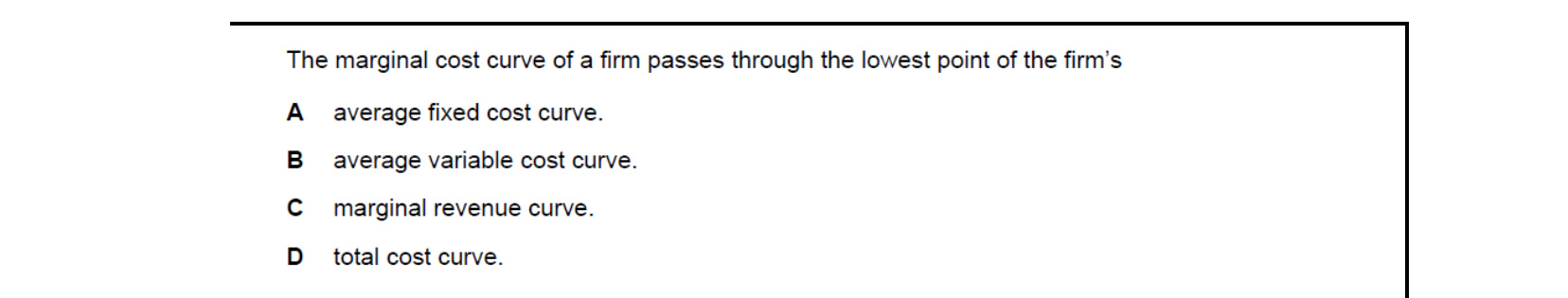
The marginal cost curve cuts the average cost curves at their lowest points. Below that point MC lies below AC and pulls average cost down; above it MC lies above AC and pulls average cost up. This applies specifically to the average variable cost curve, so MC passes through the lowest point of the AVC curve.
Average total cost = average variable cost + average fixed cost. Here AFC = ATC - AVC = $15 - $10 = $5 per unit. With total fixed cost of $1,000, output Q = TFC / AFC = 1,000 / 5 = 200 units, so the firm's output is 200 units.
34.4Long-run production function
The short run is a period of time in economics when at least one of the factors of production is fixed. The factor that tends to be easiest to change is labour; the factor that takes longest to change is capital. The short run is not defined in terms of a specific period of time — it refers to the time when not all factors of production are variable. How long that is depends on the industry: in the clothing industry it is likely to be no more than a few weeks, the time taken to install new machines and get them up and running. In other industries it will be much longer; a country building a new hydroelectric power station may take ten years to plan, install and make the station operational. This time is still referred to as the short run because capital is fixed over that period (see Figure 34.10).
All factors of production are variable in the long run. This gives the firm much greater scope to vary the respective mix of its factor inputs so that it is producing at the most efficient level. For example, if capital becomes relatively cheaper than labour, or if a new production process is invented that is likely to increase productivity, firms can reorganise the way in which they produce.
Firms must know the cost of the factors of production they use, and consider this in relation to the additional product gained from using one more unit of a factor. In the case of labour it is easy to know the costs; it is more difficult to estimate costs for other factors of production. The best combination of factors can be arrived at as their prices vary. Firms should aim to be in a position where the marginal product per unit of cost is equal across all factors of production they use:
MPA / PA = MPB / PB = MPC / PC = …
and so on for all factors of production used. For firms to be able to do this, all factors of production must be variable — which is only possible in the long run. At this combination it is impossible to lower costs further by substituting between factors.
Isoquants, isocosts and returns to scale
It is possible to derive the long-run production function for a firm by constructing an isoquant map using the principles of a production function. The map shows the different combinations of labour and capital that can be used to produce various levels of output. An isoquant map consists of a collection of isoquants for different output levels (for example, 100, 200, 300, 400 and 500 units of production). From this it is possible to read off the respective combinations of labour and capital that could produce each output level. Note that an isoquant map looks at output from a physical standpoint, not a cost standpoint; a common error is to regard isoquants as cost curves.
The shape of the isoquant map reveals returns to scale. As production rises from 100 to 200 units, relatively less extra capital and labour is required per additional unit of output: the isoquants lie close together. This is increasing returns to scale. As production expands further, increasing amounts of capital and labour are needed to produce each additional 100 units of output, and the gap between the isoquants widens. This is decreasing returns to scale. Constant returns to scale occurs in between, when proportional increases in inputs yield proportional increases in output.
In the long run, labour and capital can both be varied — the actual mix will depend on their relative prices. Isocosts are lines of constant relative costs for the factors of production; each isocost has the same slope, reflecting the price ratio of labour to capital. In deciding how to produce, the firm will be looking for the most economically efficient (least-cost) process. This is obtained by bringing isoquants and isocosts together, so linking the physical and economic sides of the production process. The point where an isocost is tangent to an isoquant represents the best combination of factors for the firm to employ. The expansion path, or long-run production function, of the firm can be shown by joining together all of the various tangency points, and is therefore useful from a longer-term planning perspective.
It is important to recognise that the above analysis is what might happen in theory. In practice:
- It is often very difficult for firms to determine their isoquants — they do not have the data or the staff know-how to be able to do this.
- It is also assumed that in the long run it is possible to switch factors of production. This may not always be as easy as the theory might indicate.
- Some employers may be reluctant to switch labour and capital — they may feel that they have a social obligation to their workforce and will therefore not alter their production plans with a change in relative factor prices.
34.5Long-run cost function
In the long run the firm can alter every input, operating at any scale. In the very long run, technological change can transform the production process and the nature of the products themselves; rapid technological progress shortens the period that counts as the short run. As a result the firm's product curves shift upwards and its cost curves shift downwards over time. Consumer electronics provides familiar illustrations of products and processes that have changed dramatically over relatively short periods.
Shape of the long-run average cost curve
The long-run average cost (LRAC) curve shows the lowest possible cost per unit at each level of output when all factors of production are variable. It is a flatter U-shape than the short-run ATC: as output rises, average cost falls (the downward-sloping section), reaches a minimum, and eventually rises again. Falling long-run average costs allow a firm to lower its prices without reducing profit.
The LRAC is built up from a series of short-run situations. As output grows, the firm expands the scale of its operations. Each scale corresponds to a different SRAC curve. The LRAC is sometimes called the envelope curve because it envelops all of the SRAC curves — each SRAC just touches the LRAC at some point. This does not mean the firm is producing at the minimum of every SRAC; it means the LRAC is the lowest attainable average cost for each output when all factors can be varied.
Minimum efficient scale
A firm operating at the lowest point of the LRAC is producing at the minimum efficient scale — the lowest level of output at which long-run average costs are minimised. The minimum efficient scale varies by industry. Where it is low relative to total market demand, many small firms can compete on equal cost terms. Where it is high relative to demand, only a few large firms can produce at the lowest possible average cost, and the market tends to be dominated by a small number of large players.
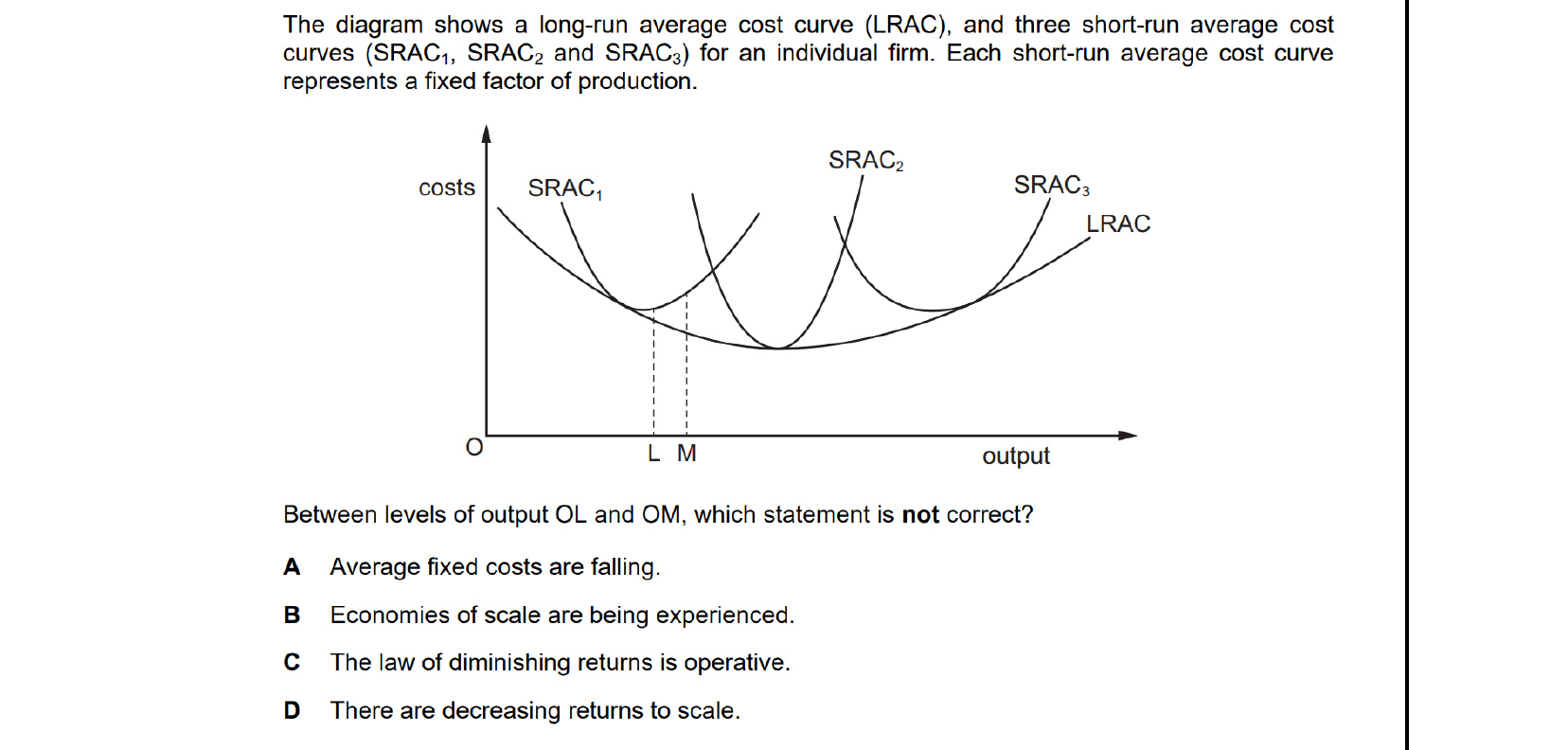
Between outputs OL and OM the LRAC is still falling, so the firm is experiencing economies of scale - returns to scale are increasing, not decreasing. Average fixed costs always fall as output rises, and diminishing returns can still operate along each SRAC. Therefore the statement that is not correct is that there are decreasing returns to scale.
34.6Internal and external economies and diseconomies of scale
The shape of the LRAC is used to explain economies of scale. A firm experiences economies of scale if costs per unit of output fall as the scale of production increases — this is shown by the downward-sloping section of the LRAC curve (see Figure 34.12).
If a firm gets increasing returns from using its factors of production, then it can produce more goods with smaller quantities of factors per unit of output. This means the firm is producing at a lower average cost. Specialisation and the division of labour are an obvious source of economies of scale, as workers become increasingly efficient in the tasks they carry out: a production line in a food processing factory is a good example, where a group of workers each contribute one part of the production process.
Beyond a certain size, a firm's costs per unit of output may instead increase as the scale of output continues to rise. This situation is one of diseconomies of scale, shown by the upward-sloping section of the LRAC curve. Note how 'scale' is used to describe production and cost concepts in the long run: this is because in the long run all factors of production are variable and so the scale of output can be increased. A common mistake is to confuse this with diminishing returns, which is a short-run concept that applies when just one factor of production is variable.
Economies of scale and decreasing average costs
Economies of scale occur when average costs decrease as the firm increases its output by increasing its size or scale of operations. They can only accrue to a firm in the long run. Internal economies of scale are the benefits gained by a firm as a result of its own decision to produce on a larger scale. They occur because the firm's output is rising proportionally faster than its inputs, meaning the firm is getting increasing returns to scale. If the increase in output is exactly proportional to the increase in inputs, the firm gets constant returns to scale and the LRAC will be horizontal. If output rises less than proportionally, the firm experiences decreasing returns to scale or diseconomies of scale — represented by any point on the LRAC curve beyond its minimum.
The advantage for a firm in benefiting from economies of scale is a reduction in the long-run average cost as the scale of output increases. This can occur in various ways:
- Technical economies refer to the advantages gained directly in the production process through more efficient production methods. Some production techniques only become viable beyond a certain level of output. Vehicle production is the result of various assembly lines; the number of finished vehicles per hour is limited by the speed of the slowest sub-process. Firms producing on a larger scale can increase the number of slow-moving lines to keep pace with the fastest, so that no resources are standing idle and the flow of finished products is higher.
- Purchasing economies. As firms increase in scale, they increase their purchasing power with suppliers. Through bulk buying, they are able to purchase supplies more cheaply, so reducing average costs. Large retailers are a classic example, using huge purchasing power to buy goods for their stores at the lowest prices. Purchasing economies can also be achieved where a retailer reduces the number of items it sells; this allows the firm to concentrate on a more limited range of goods which can be bought in bulk at discounted prices.
- Marketing economies. Large-scale firms can promote their products and pay lower rates for advertising on television, in newspapers and on social media because they purchase large amounts of air time and space. This broad category also includes savings in logistics costs — the cost of moving goods from where they are produced to where they are sold. Transport and warehousing costs can be reduced where customers require these services on a large scale. Large firms can also make savings through their IT systems: search engines, corporate websites and online retailing platforms allow customers to buy a wide range of items efficiently, and the resulting cost savings contribute to the success of huge online retailers.
- Managerial economies. In large-scale firms, managerial economies come about as a result of specialisation. Experts can be hired to manage operations, finance, human resources, sales, IT systems and so on. For small firms, these functions often have to be carried out by a multi-task manager. Cost savings are expected to accrue where specialists are employed.
- Financial economies. Large-scale firms usually have better and cheaper access to borrowed funds than smaller firms, because the perceived risk to the lender is lower.
Key concept link — Time
The benefits from economies of scale can give firms a long-run competitive advantage in the market.
External economies of scale
External economies of scale are particular benefits received by all the firms in an industry as a direct consequence of the growth of that industry. External economies of scale may be one reason for the trend towards the concentration of rival firms in the same geographical area. They can reduce long-run average costs for all firms in the industry — represented by a downward shift of the LRAC. The advantages may include the availability of a pool of skilled labour, a convenient supply of components and services from specialist producers that have grown up to provide for all firms in the area, greater access to shared knowledge and research, and better transport infrastructure provided in response to the general expansion of firms. Geographical clusters of biotechnology, electronics or lighting firms are typical examples; firms within them benefit from lower logistics costs and easier access to ideas and labour.
Diseconomies of scale
It should be made clear that there are limits to economies of scale. A firm can expand its scale of output too much, with the result that average costs start to rise and efficiency is therefore compromised. This is indicative of diseconomies of scale. The most likely source of internal diseconomies of scale lies in the problems of management co-ordination of large complex organisations and the effect that size and poor communications have on the morale of the workforce. This is one important reason why, after a period of growth, a firm may decide to split its business into two standalone companies. Another example of diseconomies of scale is where workers may feel a lack of motivation due to the repetitive nature of the work they carry out, or feel that they are a small insignificant part of a big organisation in which senior managers do not appear to have a duty of care to employees. Although not particularly visible, these are underlying reasons for an increase in costs as the firm expands its scale of operations.
In the same way that internal diseconomies of scale are possible, the excessive concentration of economic activities in a narrow geographical location can have disadvantages. External diseconomies of scale may be seen in the form of:
- traffic congestion which increases distribution costs;
- land shortages and therefore rising fixed costs;
- shortages of skilled labour and therefore rising variable costs.
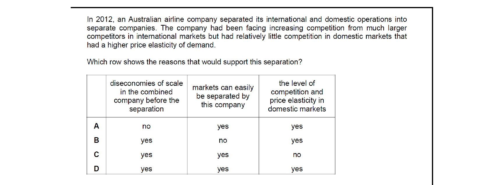
Separating the two divisions makes sense when the combined firm had grown beyond its minimum efficient scale (diseconomies of scale), when the international and domestic markets can be cleanly split into independent companies, and when the markets differ enough in competition and price elasticity to justify separate strategies. All three reasons apply here, so the correct row is yes/yes/yes.
34.7Total, average and marginal revenue
Revenue is the payment a firm receives for the goods and services it sells. It is sometimes called sales and is usually measured over a period of time such as a month or a year. Three revenue concepts mirror the three cost concepts of the short-run cost function (see Figures 34.14 and 34.15).
- Total revenue (TR) is the firm's total earnings: TR = P × Q, where P is the price and Q is the quantity sold.
- Average revenue (AR) is revenue per unit of output: AR = TR ÷ Q. For a firm selling at a single price, average revenue is the same as price.
- Marginal revenue (MR) is the extra revenue earned from selling one additional unit: MR = ΔTR ÷ ΔQ.
Price takers and price makers
The behaviour of these revenue measures depends on the type of market in which the firm operates.
In a fully competitive market the firm is a price taker: it has no control over the market price and must sell at whatever price the market sets. Its demand curve is horizontal at the market price, so AR equals the market price and MR equals AR equals price. The firm can sell as much or as little as it likes at the going price; its revenue depends only on the quantity sold. The market as a whole still has a downward-sloping demand curve.
In any other type of market the firm is a price maker — it faces a downward-sloping demand curve. If it raises output, it must lower price to sell the extra units; if it cuts output, price rises. The firm's demand curve is its average revenue curve. Because price must be reduced on every unit sold to attract the extra unit, marginal revenue is always below average revenue when the demand curve slopes downwards. The extent of the change in revenue when output changes depends on the price elasticity of demand.
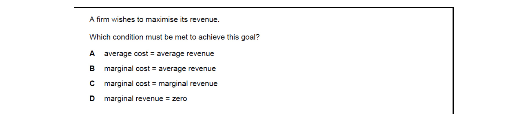
Revenue is maximised where any further unit would add less revenue than the previous one - that is, where marginal revenue equals zero. Below this output an extra unit still raises total revenue; above it, MR is negative and total revenue falls. So the condition for revenue maximisation is marginal revenue = zero.
34.8Normal, subnormal and supernormal profit
Profit is the difference between total revenue and total cost. The economist's definition of cost is wider than the accountant's because it includes the opportunity cost of any resources the entrepreneur owns and uses in the business. Capital that could have earned interest in a risk-free use, for example, must be valued and counted as a cost. Without this allowance, total costs would understate the true private cost of the activity.
An entrepreneur expects a minimum return that reflects what could have been earned elsewhere with the resources available. This minimum return is normal profit. It is the entrepreneur's reward and is included in the firm's total costs — without normal profit nothing would be produced. The firm's total costs in economic analysis therefore include normal profit, so:
Profit = Total revenue − total costs (including normal profit)
Two further concepts follow.
- Supernormal profit is profit over and above normal profit: Supernormal profit = Total profit − Normal profit. When firms in a market are earning supernormal profit, other firms have an incentive to enter the industry.
- Subnormal profit is the situation where the firm earns less than normal profit. If subnormal profit persists into the long run, the firm should leave the industry because the resources it is using could earn more elsewhere.
The key implication is that normal profit is treated as a cost, not as a residual. A firm earning exactly normal profit is breaking even in economic terms and will stay in the industry; a firm earning supernormal profit will attract new entrants; a firm earning subnormal profit in the long run will exit.
End-of-chapter practice
Past-paper questions from CIE 9708. Pick A, B, C or D. Answers are saved on this device — press Download report (PDF) at the top to save them.
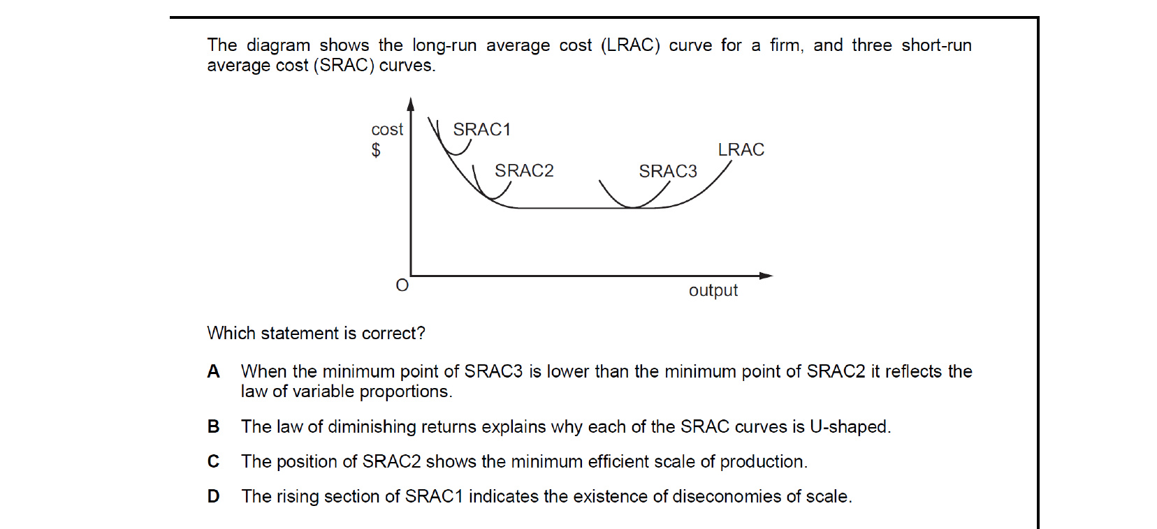
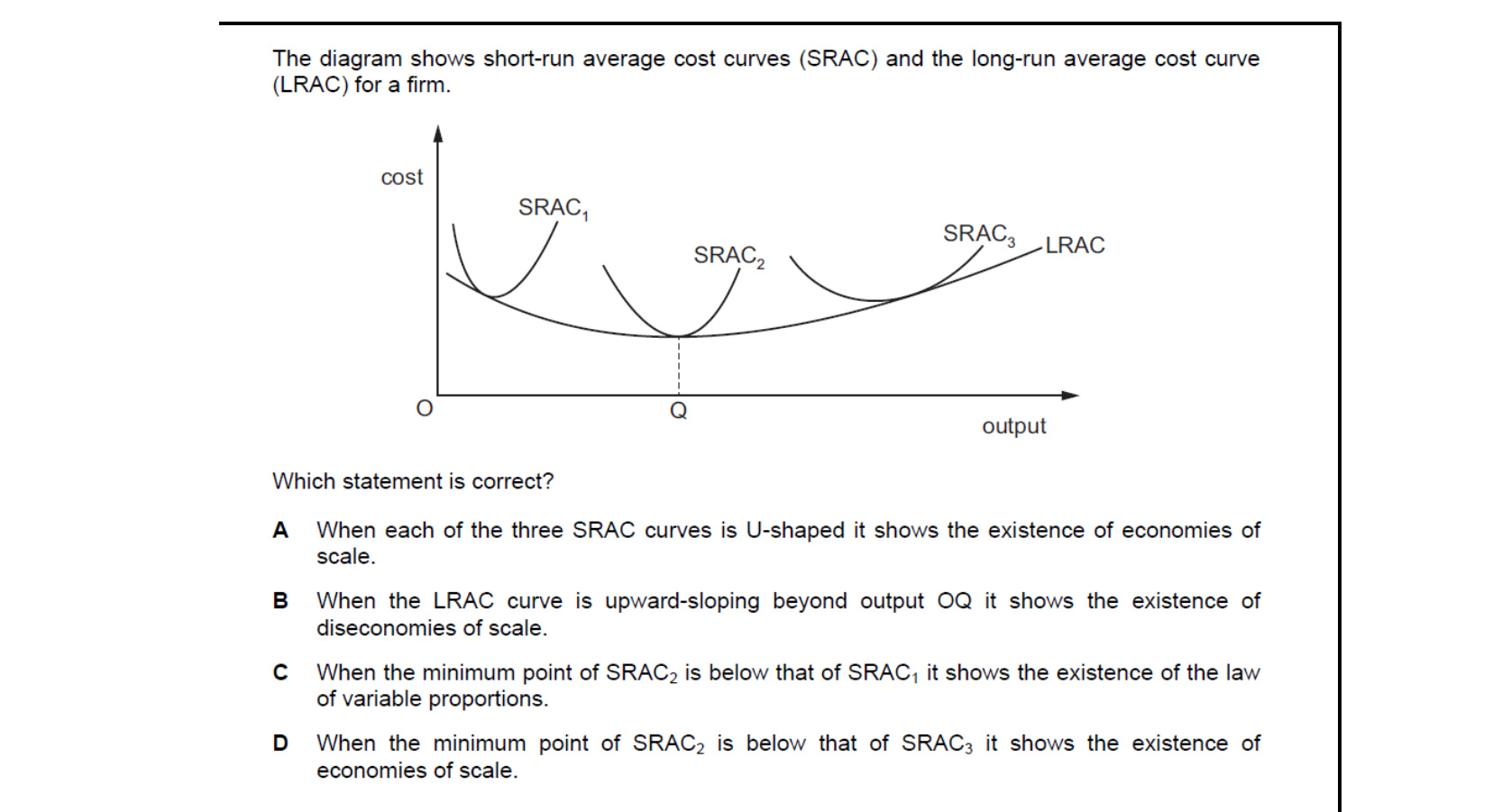
Each SRAC curve is U-shaped in the short run because of the law of diminishing returns: as output rises with at least one fixed factor, marginal product first rises then falls, dragging short-run average cost down then up. So the law of diminishing returns explains why each of the SRAC curves is U-shaped.

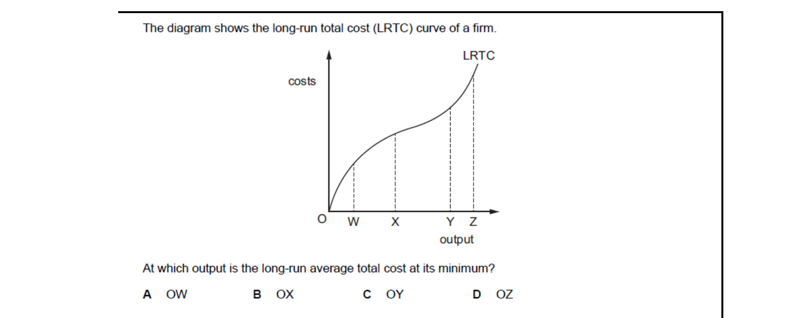
On the long-run total cost curve, long-run average cost is the slope of the ray from the origin to the curve. The minimum LRAC occurs where this ray just touches the curve - the point at which a line from the origin is tangent to LRTC. The diagram identifies this tangency at output OY.
Beyond the minimum efficient scale, further expansion raises long-run average cost - the firm experiences diseconomies of scale, normally from coordination and management problems in a very large organisation. The upward-sloping section of the LRAC beyond output OQ therefore shows the existence of diseconomies of scale.
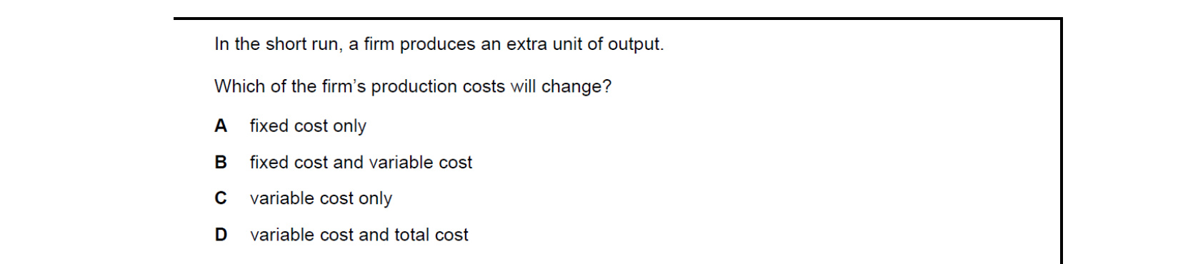
Producing an extra unit raises variable cost (more inputs are used) but fixed cost is unchanged in the short run. Because total cost is the sum of fixed and variable cost, an increase in variable cost also raises total cost. So the costs that change are variable cost and total cost.

Economies of scale cut a firm's long-run average cost as it expands; diseconomies of scale raise it. Both arise from long-run changes in the scale of operations, and both can result from management or organisational factors. What is unique to economies of scale is that they occur with decreasing average cost, while diseconomies cause average cost to rise.
Attempt the practice questions above to build your score.
Self-evaluation checklist
After studying this chapter, you should be able to:
- Explain that labour is the usual variable factor of production in the short run while all other factors of production are fixed.
- Understand the difference between total product, marginal product and average product.
- Calculate total product, marginal product and average product.
- Describe the concept of the law of diminishing returns.
- Explain the importance of the short-run cost function and the two types of short-run costs: fixed costs and variable costs.
- Calculate total cost, average fixed cost, average variable cost, average total cost, marginal cost.
- Understand that the short-run average cost curve (SRAC) and marginal cost curves are U-shaped.
- Explain that all factors of production are variable in the long run.
- Explain increasing and decreasing returns to scale.
- Explain that in the long run all inputs are variable.
- Explain why the long-run average cost curve (LRAC) is a flatter U-shaped curve.
- Explain the concept of the minimum efficient scale.
- Use the shape of the LRAC to explain internal and external economies of scale and diseconomies of scale.
- Use the total sales from a firm's output (revenue) to calculate total, average and marginal revenue.
- Understand the difference between normal, subnormal and supernormal profit.
- Calculate subnormal and super normal profit.
Want more practice? Drill this chapter's past-paper MCQs (145 questions) →