Chapter 17 — Aggregate Demand and Aggregate Supply Analysis
Cambridge International AS & A Level Economics (9708) · Unit 4.3 · 4th edition coursebook
Learning objectives
- Define the meaning of aggregate demand (AD).
- Explain the components of aggregate demand.
- Analyse the determinants of aggregate demand.
- Explain the shape of the aggregate demand curve.
- Analyse the causes of a shift in the aggregate demand curve.
- Define the meaning of aggregate supply (AS).
- Analyse the determinants of aggregate supply.
- Explain the shape of the aggregate supply curve in the short run (SRAS) and the long run (LRAS).
- Explain the causes of a shift in the AS curve in the short run (SRAS) and in the long run (LRAS).
- Identify the difference between a movement along and a shift in aggregate demand and aggregate supply.
- Explain how equilibrium is established in the AD/AS model and how the level of real output, the price level and employment are determined.
- Discuss the effects of shifts in the AD curve and the AS curve on the level of real output, the price level and employment.
Key terms
- aggregate demand (AD)
- The total demand for an economy's goods and services at a given price level in a given time period.
- consumer expenditure
- Spending by households on goods and services.
- dissaving
- Consumer expenditure exceeds income, with people or countries drawing on past savings, or borrowing.
- saving
- Income minus consumption.
- investment
- Spending on capital goods.
- government spending
- The total of local and national government expenditure on goods and services.
- net exports
- Exports minus imports.
- exchange rate
- The price of one currency in terms of another currency.
- aggregate supply (AS)
- The total output (real GDP) that producers in an economy are willing and able to supply at a given price level in a given time period.
- short-run aggregate supply (SRAS)
- The total output of an economy that will be supplied when there has not been enough time for the prices of factors of production to change.
- long-run aggregate supply (LRAS)
- The total output of a country supplied in the period when prices of factors of production have fully adjusted.
- average cost
- The cost per unit of output.
- supply-side shocks
- Large and unexpected changes in short-run aggregate supply.
- Keynesians
- People who agree with the view of the economist John Maynard Keynes (1883–1946) that government intervention is needed to achieve full employment.
- new classical economists
- Economists who think that the LRAS curve is vertical and that the economy will move towards full employment without government intervention.
- macroeconomic equilibrium
- The output and price level achieved where AD equals AS.
17.1Aggregate demand
The word 'aggregate' means total. Aggregate demand (AD) is the total spending on an economy's goods and services at a given price level over a given period of time. It captures spending by households, by firms, by the government, and by foreigners on the country's exports, less the amount spent on imports.
Aggregate demand has four components, summed by the identity AD = C + I + G + (X − M):
- Consumer expenditure (C) — spending by households on goods and services, also known as consumption.
- Investment (I) — spending by private sector firms on capital goods.
- Government spending (G) — total local and national government expenditure on goods and services.
- Net exports (X − M) — the value of exports minus the value of imports.
Each component responds to different influences, and a change in any of them will shift the AD curve.
17.2Determinants of the components of aggregate demand
Consumer expenditure
Consumer expenditure is spending by households on goods and services to satisfy current wants — food, clothing, travel, entertainment and so on. The single most important influence on consumer expenditure is the level of disposable income. When income rises, total spending usually rises with it, although richer households tend to save a larger proportion of any extra income than poorer ones.
When a person or a country is poor, most or all of disposable income has to be spent simply to meet current needs. Consumer expenditure may even exceed income, with households drawing on past savings or borrowing — a situation called dissaving. When income rises some of it can be saved, and saving is defined as disposable income minus consumer expenditure.
Other influences on consumer expenditure include:
- Distribution of income — if income becomes more equally distributed, total consumer expenditure tends to rise, because lower-income households spend a larger share of any additional income than higher-income households.
- The rate of interest — lower interest rates reduce the return from saving, make credit purchases cheaper, and leave existing borrowers with more money to spend.
- Availability of credit — easier access to loans tends to raise spending.
- Expectations — optimism about future jobs and incomes encourages spending; pessimism encourages caution.
- Wealth — a rise in the value of houses or shares tends to raise consumer expenditure.
Investment
Investment here means private sector spending by firms on capital goods such as factories, offices, machinery and delivery vehicles. Its determinants include:
- Changes in consumer demand — if firms expect to sell more, they expand capacity by buying more capital.
- The rate of interest — a lower interest rate reduces the cost of borrowing and the opportunity cost of using retained profits, and tends to raise expected demand, all of which encourage investment.
- Technology — advances in technology raise the productivity of capital goods and so make investment more attractive.
- The cost of capital goods — a fall in the price of capital equipment or in the cost of installing it tends to raise investment.
- Expectations — when firms are optimistic about the economic outlook, they invest more.
- Government policy — cuts in corporation tax or investment subsidies can encourage private sector investment.
Government investment is normally included in the government spending component, so the contribution of the public sector to AD can be seen clearly.
Government spending
Government spending includes expenditure on merit goods such as education and healthcare and on public goods such as defence — for example medicines for state hospitals, school equipment, military aircraft and government investment in infrastructure. It is shaped by:
- Government policy — if a government wants to raise economic activity, it may raise its spending.
- Tax revenue — higher tax revenue allows more spending without extra borrowing.
- Demographic change — more children raise pressure on education spending; more elderly people raise pressure on healthcare spending.
Net exports
Net exports are exports minus imports. They depend on:
- Domestic GDP — when a country's GDP rises, demand for imports usually rises and some products may be diverted from exports to the domestic market.
- GDPs of other countries — when incomes rise abroad, demand for the country's exports tends to increase.
- Relative price and quality competitiveness — improvements in productivity, quality or marketing of domestically produced goods raise exports.
- The exchange rate — a fall in the exchange rate makes exports cheaper abroad and imports dearer at home. If demand for exports and imports is elastic, export revenue rises and import expenditure falls, so net exports rise.
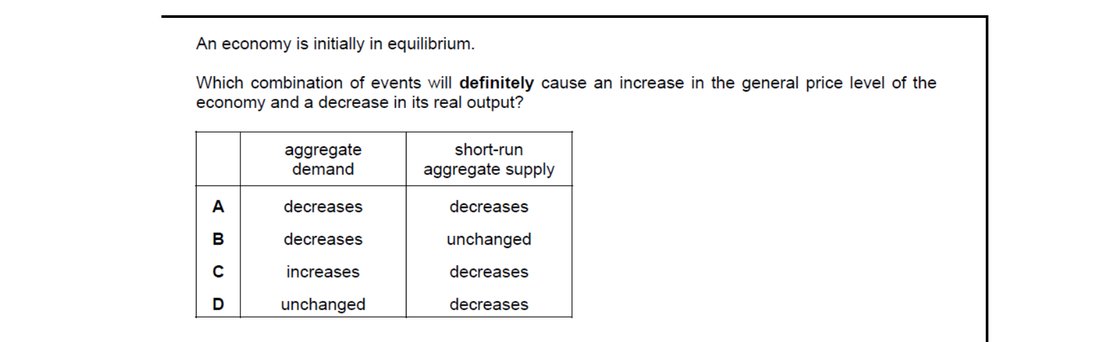
A combination that definitely raises the price level while reducing real output requires AD to be at least unchanged and SRAS to fall. Option D — aggregate demand unchanged and short-run aggregate supply decreasing — gives exactly this: the SRAS leftward shift pushes the price level up and real output down along an unchanged AD curve.
17.3The aggregate demand curve
The aggregate demand curve (see Figure 17.3) shows the different quantities of total demand for an economy's products at different price levels. It slopes downwards from left to right: a rise in the price level causes a contraction in aggregate demand and a fall in the price level causes an extension. On the axes, the vertical axis measures the general price level (not the price of a single product) and the horizontal axis measures real GDP (not the quantity of a single product).
The downward slope of AD looks superficially like the demand curve for a single product, but the reasoning is different. A product's demand curve traces the effect of a change in its relative price while other prices are held constant; consumers switch towards or away from substitutes. Along the AD curve almost all prices are moving together, so the explanation must come from elsewhere. There are three reasons:
- The wealth effect — a higher price level reduces the purchasing power of money held in bank accounts and other financial assets, so the real value of wealth falls and spending falls with it.
- The international effect — a higher domestic price level makes exports less price-competitive and imports more attractive, reducing net exports.
- The interest rate effect — a higher price level raises demand for money to pay for transactions; this pushes up the rate of interest, which discourages consumption and investment.
Shifts in the aggregate demand curve
A change in the price level moves the economy along the AD curve. A change in any non-price-level influence shifts the curve, as shown in Figure 17.4. A shift to the right indicates an increase in aggregate demand; a shift to the left indicates a decrease. Examples of changes that increase aggregate demand include:
- Consumer expenditure — a rise in consumer confidence, a cut in income tax, an increase in wealth, a rise in the money supply, or an increase in the population.
- Investment — a rise in business confidence, a cut in corporate tax, or advances in technology.
- Government spending — a desire to stimulate economic activity or to win political support.
- Net exports — a fall in the exchange rate, a rise in the quality of domestically produced products, or an increase in incomes abroad.
The opposite changes shift AD to the left.
When drawing an AD curve we hold other determinants of spending constant and vary only the general price level. The money supply is one of those determinants — a change in it would shift the curve, so it is assumed constant. Tax revenue and unemployment vary endogenously with income, and interest rates may also change along the curve.
17.4Aggregate supply
Aggregate supply (AS) is the total planned output of all the producers in the country. Economists usually distinguish between two time horizons. Short-run aggregate supply (SRAS) is the output supplied in a period in which the prices of factors of production have not had time to adjust to changes in aggregate demand and the price level. Long-run aggregate supply (LRAS) is the output supplied once the prices of factors of production have fully adjusted.
The short-run aggregate supply curve
The SRAS curve (see Figure 17.5) slopes upwards from left to right: as the price level rises, producers are willing and able to supply more goods and services. Three reasons explain this positive relationship:
- The profit effect — as output prices rise but input prices such as wages remain unchanged in the short run, the gap between selling prices and factor costs widens, raising profits and encouraging more production.
- The cost effect — even with input prices fixed along an SRAS curve, average cost tends to rise as output expands, because firms have to pay overtime, recruit additional workers, and so on. Higher prices are needed to cover these extra unit costs.
- The misinterpretation effect — producers may confuse a general rise in the price level with a rise in their own product's relative price, and so raise output thinking that demand for their particular product has risen.
Shifts in the short-run aggregate supply curve
A change in the price level produces a movement along the SRAS curve. There are four main causes of a shift in SRAS:
- A change in the price of factors of production — a rise in wage rates not matched by higher productivity, or a rise in raw material costs, shifts SRAS to the left.
- A change in taxes on firms — a reduction in corporation tax or in indirect taxes shifts SRAS to the right.
- A change in factor productivity or quality of resources — a rise in labour or capital productivity raises aggregate supply in both the short run and the long run.
- A change in the quantity of resources — in the short run, supply of inputs can be hit by supply-side shocks such as natural disasters. Such shocks may not have a large impact on productive potential in the long run, but the factors that raise the quantity of resources in the long run will also raise SRAS.
The shape of the long-run aggregate supply curve
The LRAS curve shows the relationship between real GDP and the price level once input prices have had time to adjust. There are two views of its shape.
The Keynesian view. Keynesians draw LRAS as perfectly elastic at low rates of output, then upward sloping over a range of output, and finally perfectly inelastic (see Figure 17.7). They emphasise that, in the long run, an economy can operate at any level of output and need not be at full capacity. When output and employment are low, firms can attract extra resources without raising their prices — for example, when unemployment is high the offer of a job can be enough to attract workers without a higher wage. As output rises further, firms experience shortages and start bidding up wages, raw material prices and the price of capital equipment. At the maximum output the economy can produce with existing resources, the LRAS curve becomes vertical.
The new classical view. New classical economists draw LRAS as a vertical line (see Figure 17.8), on the view that in the long run the economy will always operate at full capacity. A rise in aggregate demand may raise output in the short run by encouraging firms to make more intensive use of existing resources — overtime, longer running of capital equipment between maintenance — but this intensive use raises costs of production over time. The SRAS curve shifts back, and output returns to its long-run level at a higher price level.
The distinction between these two views is a useful evaluative point in answering questions such as 'discuss whether a rise in aggregate demand will cause inflation'. On a Keynesian LRAS, the effect on the price level depends on where the economy is operating; on a new classical LRAS, the long-run effect is entirely on prices, not output.
Shifts in the LRAS curve
Keynesian and new classical economists agree about what shifts LRAS: changes in the quantity and/or quality of resources. Both raise the productive potential of the economy.
Causes of an increase in the quantity of resources in the long run include:
- Net immigration of people of working age, which increases the labour force.
- A rise in the retirement age, which increases the labour force as life expectancy rises.
- More women entering the labour force; the female participation rate varies widely between countries.
- Net investment — when gross investment exceeds depreciation, the capital stock grows.
- Discovery of new resources such as new oil fields or gold mines.
- Land reclamation, which can add to a country's usable land area.
The two main causes of an increase in the quality of resources are:
- Improved education and training, which raise the skills of workers and so raise labour productivity.
- Advances in technology, which both reduce costs of production and increase productive capacity.
An outward (rightward) shift of AD requires a rise in C, I, G or net exports at every price level. A depreciation of the currency makes exports cheaper abroad and imports dearer at home, raising (X minus M) and so shifting AD outward. A fall in the price level is a movement along AD, while less competitiveness or a tighter money supply would each shift AD inward.
17.5Macroequilibrium and disequilibrium
The equilibrium level of output and the price level are determined where aggregate demand equals aggregate supply. Macroeconomic equilibrium is shown by the intersection of the AD and AS curves (see Figure 17.11).
If the price level is below the equilibrium level, total demand exceeds total supply: shortages push prices up until equilibrium is reached. If the price level is above the equilibrium level, some goods and services go unsold and firms cut their prices until equilibrium is restored.
Changes in AD and AS move the economy to a new macroeconomic position. The size and direction of the change, and the economy's initial position, all matter. If an economy is operating below but close to its productive potential, an increase in aggregate demand may raise output, employment and the price level. If it is operating with a great deal of spare capacity, the same increase may raise output and employment with little effect on the price level. If it is operating at or near full capacity, most of the increase may show up as a higher price level rather than higher output. Some variables — including investment, net immigration and government spending on education — shift both the AD and the AS curves.
Key concept link — Equilibrium and disequilibrium
Section 17.5 refers to macroeconomic equilibrium. Economists study what the current macroeconomic equilibrium is, why it has changed in recent times and what the desired level of macroeconomic equilibrium would be.
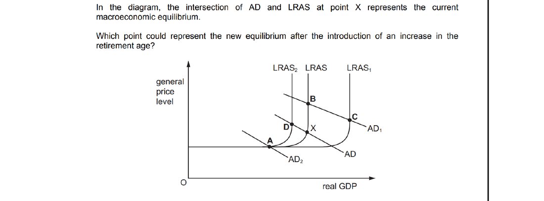
Raising the retirement age keeps more workers in the labour force, expanding the economy's productive capacity. LRAS therefore shifts to the right while AD is essentially unchanged in the long run. The new equilibrium lies on the rightward LRAS, with higher real GDP and a lower general price level — point C.
End-of-chapter practice
Past-paper questions from CIE 9708. Pick A, B, C or D. Answers are saved on this device — press Download report (PDF) at the top to save them.
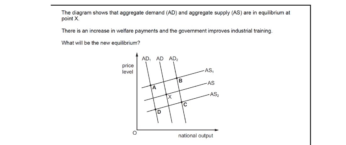
Higher welfare payments raise household incomes and consumption, shifting AD to the right. Improved industrial training raises labour productivity, shifting LRAS (and SRAS) to the right. With both AD and AS expanding, real output rises clearly while the price-level effect is muted — the new equilibrium lies to the right at point C.
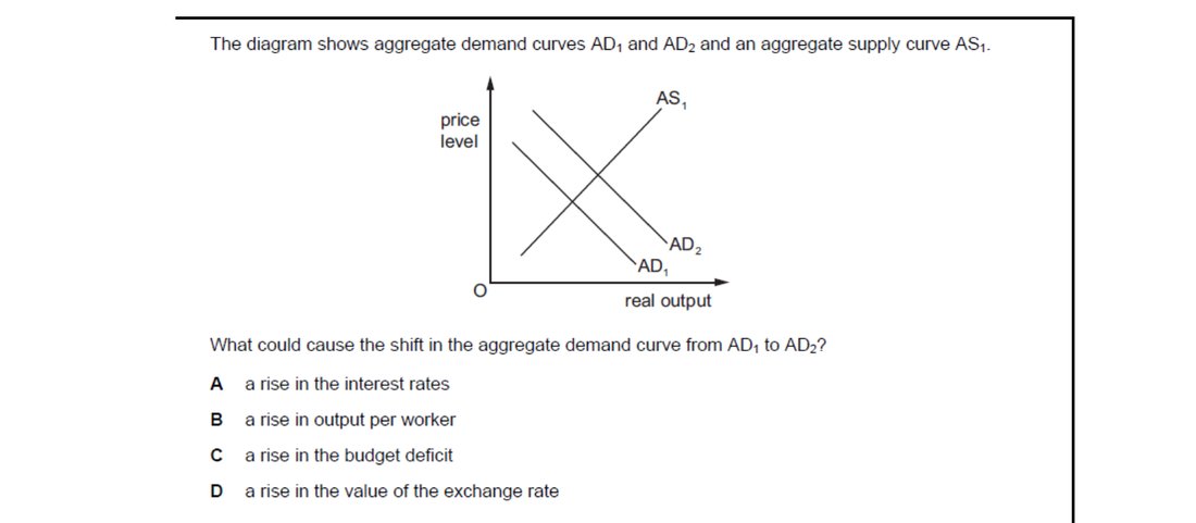
An outward shift of AD requires a rise in one of its components. A larger budget deficit means either higher government spending or lower taxes, both of which raise AD directly. Higher interest rates and currency appreciation would each shift AD inward, and a rise in output per worker affects AS rather than AD.
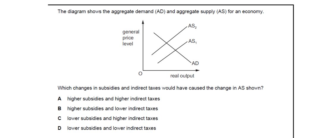
A leftward shift of AS reflects higher production costs. Indirect taxes add directly to firms' costs of supplying output, while subsidies reduce them. So raising indirect taxes and cutting subsidies both push costs up at every output level, shifting AS to the left exactly as the diagram shows.
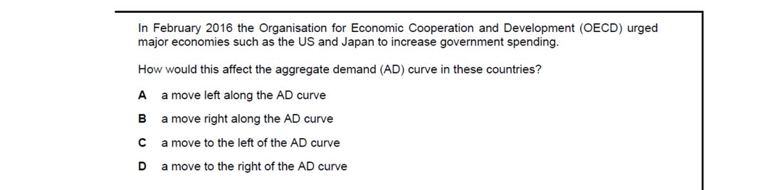
An increase in government spending is a rise in the G component of AD, so it shifts the entire AD curve outward — to the right. Movements along AD only occur when the price level itself changes; here it is a change in autonomous expenditure, so the curve shifts.
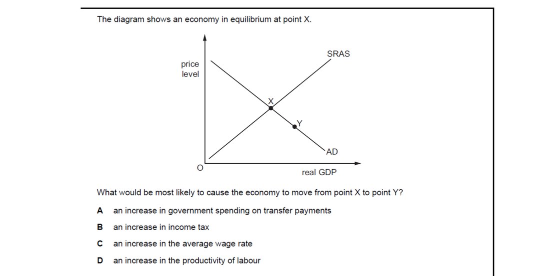
Moving from X to Y reflects higher real GDP with a lower price level — a rightward shift in aggregate supply. An increase in labour productivity raises output per worker, lowering unit costs and expanding productive capacity, so both SRAS and LRAS shift right. The other options either reduce AD or raise costs, and none generates higher output with lower prices.
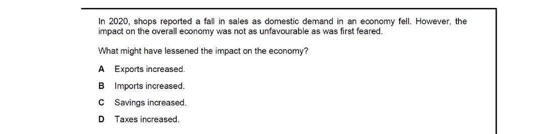
When domestic demand falls, the loss to AD can be offset by a rise in another component. An increase in exports raises (X minus M), boosting AD from outside the domestic economy. The other options either subtract from AD (more imports, more saving) or remove spending power (higher taxes), so they would worsen rather than lessen the impact.
Attempt the practice questions above to build your score.
Self-evaluation checklist
After studying this chapter, you should be able to:
- Explain that aggregate demand (AD) consists of consumer expenditure (C), investment (I), government spending (G), net exports (X − M).
- Identify the determinants that influence the components of AD.
- Understand that the AD curve slopes down from left to right and shows the different quantities of total demand for the economy's products at different prices.
- Analyse the causes of a shift to the right in the AD curve.
- Explain that aggregate supply (AS) is the total output that producers in a country are willing and able to supply at a given price level in a given time period.
- Explain why the SRAS curve is upward sloping.
- Analyse the causes of a shift in the SRAS curve.
- Analyse the causes of a shift in the LRAS curve.
- Differentiate between the reasons for a movement along the AD or AS curve and a shift in the AD or AS curve.
- Explain how equilibrium is established in the AD/AS model when aggregate demand equals aggregate supply.
- Analyse the effects of shifts in the AD curve and the AS curve on the level of real output, the price level and employment.
Want more practice? Drill this chapter's past-paper MCQs (112 questions) →