Chapter 9 — Price Elasticity of Supply
Cambridge International AS & A Level Economics (9708) · Unit 2.3 · 4th edition coursebook
Learning objectives
- Define and calculate price elasticity of supply (PES).
- Interpret elastic, inelastic, unit elastic, perfectly elastic and perfectly inelastic supply.
- Identify the determinants of PES.
- Apply PES to explain the speed and depth of market adjustment.
Key terms
- price elasticity of supply (PES)
- The responsiveness of quantity supplied to a change in price, measured as %ΔQs / %ΔP.
- elastic supply
- PES > 1 — supply responds more than proportionately to price changes.
- inelastic supply
- PES < 1 — supply responds less than proportionately to price changes.
- perfectly elastic supply
- PES = ∞ — horizontal supply curve.
- perfectly inelastic supply
- PES = 0 — vertical supply curve. Quantity does not respond to price.
- spare capacity
- Unused productive capacity that firms can deploy quickly without major investment.
9.1Defining and calculating PES
Price elasticity of supply is calculated as %ΔQs / %ΔP. Because both quantity and price move in the same direction (law of supply), PES is positive.
Categories:
- PES > 1 → elastic.
- PES < 1 → inelastic.
- PES = 1 → unit elastic. The general contrast between an inelastic and an elastic supply curve is shown in Figure 9.2.
- PES = ∞ → perfectly elastic (horizontal curve).
- PES = 0 → perfectly inelastic (vertical curve). The two extreme cases are shown in Figure 9.3.

PES = %change in Qs / %change in P. Price rises from $2.00 to $2.20, a 10% increase. Short-run PES of 0.8 means Qs rises 8% (8000), giving 108000; long-run PES of 1.4 means Qs rises 14% (14000), giving 114000. The additional increase between short and long run is 114000 - 108000 = 6000. Option A is correct; the others mistake the cumulative or base figure.
9.2Determinants of PES
Supply tends to be more elastic when:
- Firms have spare capacity — extra output is cheap to ramp up.
- Stocks of finished goods or raw materials are high — they can be released quickly.
- Production is quick — manufacturing typically more elastic than agriculture.
- Inputs are easy to find at short notice — labour, raw materials, factor mobility.
- Time period is longer — long-run supply is generally more elastic than short-run.
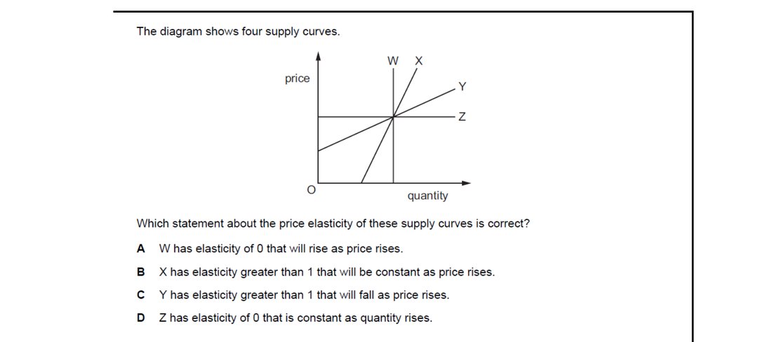
On a straight-line supply curve cutting the price axis, PES exceeds 1 and decreases as price rises. Curve Y passes through the price axis, so it is elastic but its PES falls as we move up. Option C captures this. Option A confuses a vertical curve, B implies constant elasticity along a non-origin line, and D mistakes a vertical line for one whose elasticity is undefined/infinite.
9.3Why PES matters for market adjustment
When demand shifts in a market with elastic supply, most of the adjustment occurs through quantity — price moves little. When supply is inelastic, most of the adjustment occurs through price — quantity barely changes.
Agricultural markets often show inelastic short-run supply (crops take months or years to grow), making them price-volatile. Manufacturing markets typically have more elastic supply (factories scale up faster), so price absorbs less of the demand shock. Figure 9.4 shows the same demand shift applied to supply curves of different PES, making the split between price and quantity adjustment visible.
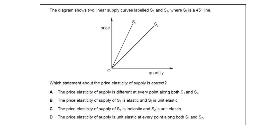
Any straight-line supply curve drawn through the origin – including a 45-degree line – has unit elasticity at every point, because price and quantity rise in equal proportion. Option D – both curves are unit elastic at every point – follows directly. Option A confuses non-origin lines, and B and C wrongly classify origin-based lines as elastic or inelastic.
End-of-chapter practice
Past-paper questions from CIE 9708. Pick A, B, C or D. Answers are saved on this device — press Download report (PDF) at the top to save them.
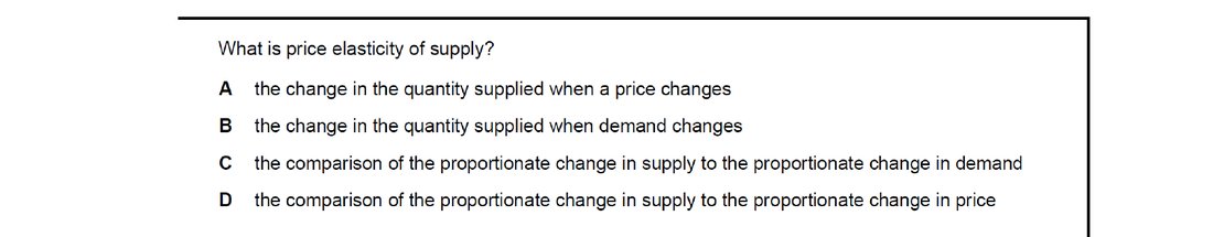
Price elasticity of supply measures the responsiveness of quantity supplied to a change in price, expressed as percentages. Option D – the proportionate change in supply compared with the proportionate change in price – is the standard definition. Option A omits proportionality, B confuses PES with a quantity-demand link, and C wrongly references demand rather than price.
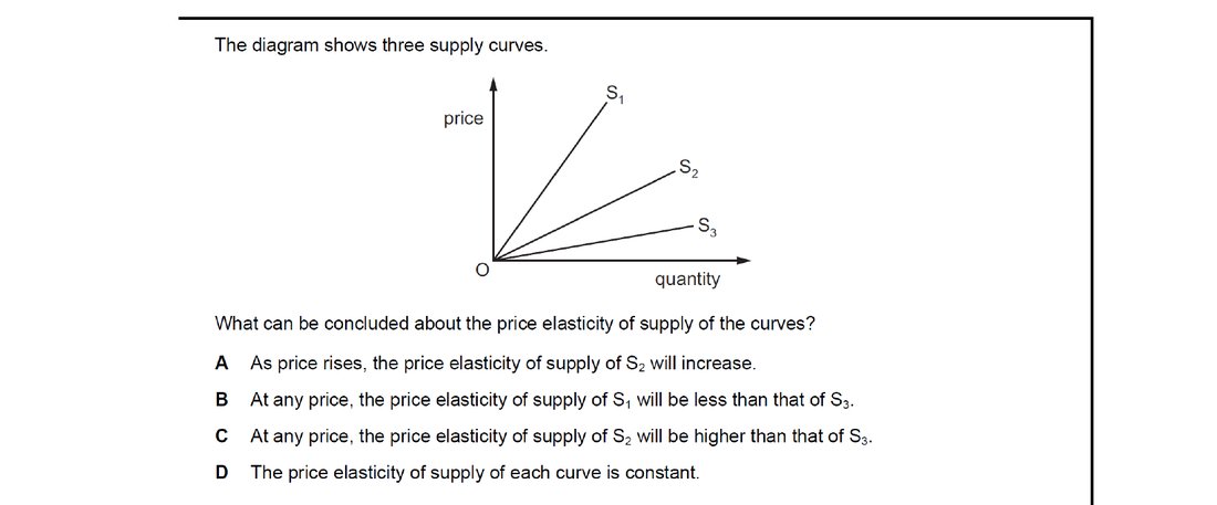
When a supply curve is a straight line through the origin, including a 45-degree line, PES equals 1 at every point. The three curves shown all start at the origin, so their PES is constant. Option D – PES of each curve is constant – is correct. A and B incorrectly imply varying elasticity, and C ranks elasticities that are in fact identical.

As the time period lengthens, more factors of production become variable: firms can build capacity, recruit workers and reorganise. Supply therefore becomes more responsive to price, so PES rises with time. Option B states exactly this. Option A is false (PES does change), C overstates the momentary case (which is typically zero), and D reverses the long-run effect.

Using S = 10 + 10P: at P = 1, S = 20; at P = 2, S = 30. Quantity rises by 10, a 50% increase; price rises 100%. PES = 50/100 = 0.5. Option A is correct. Options B-D mistakenly use either the slope or the absolute change rather than percentage changes from the initial values.

Agricultural crops such as wheat take many months to grow, so producers cannot respond quickly to price changes in the short run, making supply inelastic. Option D – the long time required to produce additional output – captures this biological lag. Options A, B and C describe responses or technologies that increase, not decrease, supply elasticity.
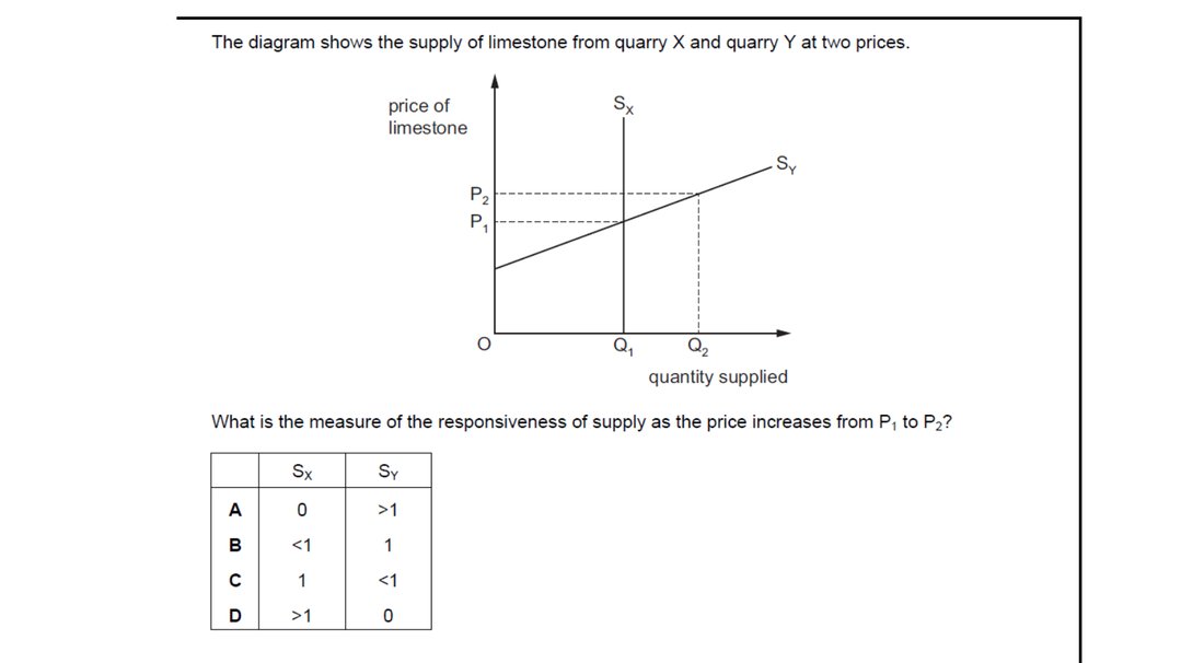
PES = %change in Qs / %change in P. Quarry X shows quantity rising while price rises – a positive but proportional response that the diagram implies is greater than 1 (elastic). Quarry Y's quantity is unchanged at the higher price, indicating zero elasticity. Option A – X > 1 and Y = 0 – matches this; the other rows misread one or both curves.

PES measures how much quantity supplied responds to a change in the good's own price. Option C – how much supply changes when there is a change in price – is the textbook description. Option A reverses cause and effect, B substitutes demand for price (a different concept), and D refers to a substitute's price (cross supply, not own-price elasticity).
Attempt the practice questions above to build your score.
Self-evaluation checklist
After studying this chapter, you should be able to:
- Calculate PES from data and classify the supply curve.
- Identify the determinants of PES.
- Predict the price and quantity effects of a demand shift given the elasticity of supply.
Want more practice? Drill this chapter's past-paper MCQs (92 questions) →